The Accuracy of Computational Results from Wolfram Mathematica in the Context of Summation in Trigonometry

Abstract

This article explores the accessibility of symbolic computations, such as using the Wolfram Mathematica environment, in promoting the shift from informal experimentation to formal mathematical justifications. We investigate the accuracy of computational results from mathematical software in the context of a certain summation in trigonometry. In particular, the key issue addressed here is the calculated sum ${\sum }_{n=0}^{44}{\tan \left(1+4n\right)}^{°}.$ This paper utilizes Wolfram Mathematica to handle the irrational numbers in the sum more accurately, which it achieves by representing them symbolically rather than using numerical approximations. Can we rely on the calculated result from Wolfram, especially if almost all the addends are irrational, or must the students eventually prove it mathematically? It is clear that the problem can be solved using software; however, the nature of the result raises questions about its correctness, and this inherent informality can encourage a few students to seek viable mathematical proofs. In this way, a balance is reached between formal and informal mathematics.

1. Introduction

The purpose of this article is to illustrate how the accessibility of symbolic computations, such as the Wolfram Mathematica environment, facilitates the shift from relying on informal experiments to providing justifications for results using mathematical methods. We ask how mathematical software can help motivate high school students to further explore mathematics [1].

If we give the students a problem, they can solve it by means of software, the produced result may raise some questions about its correctness or accuracy. Furthermore, this could motivate the students to attempt to prove the result mathematically.

An example of such a problem is one where the solution is a specific numerical value, and the accuracy of this value depends on the precision of the performed calculations. It turns out that such a suitable problem could be a sum of irrational numbers.

Let us look at the following sum:

$$\sum _{n=0}^{44}{\tan (1+4n)}^{°}.$$

First, we need to say something about how the irrationality of the intermediate results affects the accuracy of the overall result calculated by a program.

Mathematical software has revolutionized the way we approach complex calculations, making it easier and more efficient to solve intricate mathematical problems [2].

However, these software tools have their limitations. One such limitation lies in their inability to compute exact results when dealing with irrational numbers. When mathematical software encounters an irrational number, it attempts to approximate it by truncating or rounding the decimal representation. These approximations introduce errors, which can be magnified when multiple operations are performed on these approximated values. Consequently, the computed results deviate from the exact values, leading to inaccuracies in complex calculations.

To mitigate the limitations of mathematical software, alternative approaches can be used. One of these approaches is symbolic computation, which manipulates mathematical expressions symbolically rather than relying on numerical approximations [2,3]. Symbolic computation systems, such as Wolfram Mathematica, Maple, MATLAB, etc., can handle irrational numbers more accurately by representing them symbolically instead of as approximations.

In the case of calculating a sum of irrational numbers, mathematical software can sometimes produce correct results because the errors introduced by approximating individual irrational numbers cancel each other out or are small enough to be negligible. This cancellation of errors can occur, for example, due to the properties of the numbers involved or the specific algorithm used for the computation.

It is important to note that this ability to compute correct results in some cases does not negate the inherent limitations of mathematical software when dealing with irrational numbers. The accuracy of the results depends on various factors, including the algorithm used, the precision of the calculations, and the properties of the numbers involved. In more complex calculations or when dealing with a larger number of irrational numbers, the limitations of mathematical software in handling exact results for irrational numbers become more evident.

While mathematical software may sometimes produce correct results when dealing with a sum of irrational numbers, this is due to the algorithms used and the properties of the numbers involved. The software does not compute the exact values of the irrational numbers but rather provides accurate approximations that minimize error. The limitations of mathematical software in handling exact results for irrational numbers still exist and must be considered in situations where precision is necessary [4].

2. Materials and Methods of Problem Solving

We start with the following problem.

What is the exact value of ${\sum }_{n=0}^{44}{\tan (1+4n)}^{°}$ = $\tan 1^{°}+\tan 5^{°}+\tan 9^{°}+\cdots +\tan {177}^{°}?$

Sooner or later, the students stop looking for relations using trigonometric identities and try some kind of software to find the sum.

Let us assume that MS Excel is employed by some of the students.

If the sum is displayed to a maximum of 12 decimal places, the result will always be 45.000000000000.

Since the students know that at least some of these addends are irrational numbers (or rather, they probably know that the values of all other addends than ${\tan 45}^{°}$ are irrational) [5], this exact number 45 will probably surprise them. It occurs to them to increase the number of displayed decimal places, and from 13 onwards, they will already receive results like 44.9999999999997. Hence, they will be satisfied with the following answer:

$$\sum _{n=0}^{44}{\tan (1+4n)}^{°}\doteq 45.$$

That is, the sum equals “about” 45, while the exact value of 45 will never come out; it is just a rounded value. For the students to think about this sum further, we let them enter it into the Wolfram Mathematica program.

Here, they find (if they display the overall result, for example, up to 300 decimal places) that the sum is

45.000000000000000000000000000000000000000000000000000000000000000000000000000000000000000000000000000000000000000000000000000000000000000000000000000000000000000000000000000000000000000000000000000000000000000000000000000000000000000000000000000000000000000000000000000000000000000000000000000000000000.

Perhaps the students think that the sum is, in fact, exactly 45. How can it be proven? From what they have carried out so far, it is clear that the computer cannot help here [6].

Just mathematics itself can give them the proof!

So, they are in a situation where the use of ICT has forced them to consider mathematics as a tool and in more detail.

First, let us show what the students can see in Wolfram Mathematica.

What is the value of the sum ${\sum }_{n=0}^{44}{\tan (1+4n)}^{°}?$

Mathematica prints the following:

Explanation	e.g.,
# of the addend	3
Angle value	9°
tan (angle)°	0.1583844403
Partial sum of angle degrees	0.2633281688

$\#: 1 \mathrm{Angle}: 1^{\circ }\mathrm{Tan}[ 1^{\circ } ]: 0.01745506493 \mathrm{Partial} \mathrm{sum} \mathrm{of} 1 \mathrm{degrees}: 0.01745506493$

$\#: 2 \mathrm{Angle}: 5^{\circ }\mathrm{Tan}[ 5^{\circ } ]: 0.08748866353 \mathrm{Partial} \mathrm{sum} \mathrm{of} 5 \mathrm{degrees}: 0.1049437285$

$\#: 3 \mathrm{Angle}: 9^{\circ }\mathrm{Tan}[ 9^{\circ } ]: 0.1583844403 \mathrm{Partial} \mathrm{sum} \mathrm{of} 9 \mathrm{degrees}: 0.2633281688$

$\#: 4 \mathrm{Angle}: {13}^{\circ }\mathrm{Tan}[ {13}^{\circ } ]: 0.2308681911 \mathrm{Partial} \mathrm{sum} \mathrm{of} 13 \mathrm{degrees}: 0.4941963599$

$\#: 5 \mathrm{Angle}: {17}^{\circ }\mathrm{Tan}[ {17}^{\circ } ]: 0.3057306815 \mathrm{Partial} \mathrm{sum} \mathrm{of} 17 \mathrm{degrees}: 0.7999270414$

$\#: 6 \mathrm{Angle}: {21}^{\circ }\mathrm{Tan}[ {21}^{\circ } ]: 0.3838640350 \mathrm{Partial} \mathrm{sum} \mathrm{of} 21 \mathrm{degrees}: 1.183791076$

$\#: 7 \mathrm{Angle}: {25}^{\circ }\mathrm{Tan}[ {25}^{\circ } ]: 0.4663076582 \mathrm{Partial} \mathrm{sum} \mathrm{of} 25 \mathrm{degrees}: 1.650098735$

$\#: 8 \mathrm{Angle}: {29}^{\circ }\mathrm{Tan}[ {29}^{\circ } ]: 0.5543090515 \mathrm{Partial} \mathrm{sum} \mathrm{of} 29 \mathrm{degrees}: 2.204407786$

$\#: 9 \mathrm{Angle}: {33}^{\circ }\mathrm{Tan}[ {33}^{\circ } ]: 0.6494075932 \mathrm{Partial} \mathrm{sum} \mathrm{of} 33 \mathrm{degrees}: 2.853815379$

$\#: 10 \mathrm{Angle}: {37}^{\circ }\mathrm{Tan}[ {37}^{\circ } ]: 0.7535540501 \mathrm{Partial} \mathrm{sum} \mathrm{of} 37 \mathrm{degrees}: 3.607369429$

$\#: 11 \mathrm{Angle}: {41}^{\circ }\mathrm{Tan}[ {41}^{\circ } ]: 0.8692867378 \mathrm{Partial} \mathrm{sum} \mathrm{of} 41 \mathrm{degrees}: 4.476656167$

$\#: 12 \mathrm{Angle}: {45}^{\circ }\mathrm{Tan}[ {45}^{\circ } ]: 1.000000000 \mathrm{Partial} \mathrm{sum} \mathrm{of} 45 \mathrm{degrees}: 5.476656167$

$\#: 13 \mathrm{Angle}: {49}^{\circ }\mathrm{Tan}[ {49}^{\circ } ]: 1.150368407 \mathrm{Partial} \mathrm{sum} \mathrm{of} 49 \mathrm{degrees}: 6.627024574$

$\#: 14 \mathrm{Angle}: {53}^{\circ }\mathrm{Tan}[ {53}^{\circ } ]: 1.327044822 \mathrm{Partial} \mathrm{sum} \mathrm{of} 53 \mathrm{degrees}: 7.954069396$

$\#: 15 \mathrm{Angle}: {57}^{\circ }\mathrm{Tan}[ {57}^{\circ } ]: 1.539864964 \mathrm{Partial} \mathrm{sum} \mathrm{of} 57 \mathrm{degrees}: 9.493934360$

$\#: 16 \mathrm{Angle}: {61}^{\circ }\mathrm{Tan}[ {61}^{\circ } ]: 1.804047755 \mathrm{Partial} \mathrm{sum} \mathrm{of} 61 \mathrm{degrees}: 11.29798212$

$\#: 17 \mathrm{Angle}: {65}^{\circ }\mathrm{Tan}[ {65}^{\circ } ]: 2.144506921 \mathrm{Partial} \mathrm{sum} \mathrm{of} 65 \mathrm{degrees}: 13.44248904$

$\#: 18 \mathrm{Angle}: {69}^{\circ }\mathrm{Tan}[ {69}^{\circ } ]: 2.605089065 \mathrm{Partial} \mathrm{sum} \mathrm{of} 69 \mathrm{degrees}: 16.04757810$

$\#: 19 \mathrm{Angle}: {73}^{\circ }\mathrm{Tan}[ {73}^{\circ } ]: 3.270852618 \mathrm{Partial} \mathrm{sum} \mathrm{of} 73 \mathrm{degrees}: 19.31843072$

$\#: 20 \mathrm{Angle}: {77}^{\circ }\mathrm{Tan}[ {77}^{\circ } ]: 4.331475874 \mathrm{Partial} \mathrm{sum} \mathrm{of} 77 \mathrm{degrees}: 23.64990659$

$\#: 21 \mathrm{Angle}: {81}^{\circ }\mathrm{Tan}[ {81}^{\circ } ]: 6.313751515 \mathrm{Partial} \mathrm{sum} \mathrm{of} 81 \mathrm{degrees}: 29.96365811$

$\#: 22 \mathrm{Angle}: {85}^{\circ }\mathrm{Tan}[ {85}^{\circ } ]: 11.43005230 \mathrm{Partial} \mathrm{sum} \mathrm{of} 85 \mathrm{degrees}: 41.39371041$

$\#: 23 \mathrm{Angle}: {89}^{\circ }\mathrm{Tan}[ {89}^{\circ } ]: 57.28996163 \mathrm{Partial} \mathrm{sum} \mathrm{of} 89 \mathrm{degrees}: 98.68367204$

$\#: 24 \mathrm{Angle}: {93}^{\circ }\mathrm{Tan}[ {93}^{\circ } ]: -19.08113669 \mathrm{Partial} \mathrm{sum} \mathrm{of} 93 \mathrm{degrees}: 79.60253535$

$\#: 25 \mathrm{Angle}: {97}^{\circ }\mathrm{Tan}[ {97}^{\circ } ]: -8.144346428 \mathrm{Partial} \mathrm{sum} \mathrm{of} 97 \mathrm{degrees}: 71.45818893$

$\#: 26 \mathrm{Angle}: {101}^{\circ }\mathrm{Tan}[ {101}^{\circ } ]: -5.144554016 \mathrm{Partial} \mathrm{sum} \mathrm{of} 101 \mathrm{degrees}: 66.31363491$

$\#: 27 \mathrm{Angle}: {105}^{\circ }\mathrm{Tan}[ {105}^{\circ } ]: -3.732050808 \mathrm{Partial} \mathrm{sum} \mathrm{of} 105 \mathrm{degrees}: 62.58158410$

$\#: 28 \mathrm{Angle}: {109}^{\circ }\mathrm{Tan}[ {109}^{\circ } ]: -2.904210878 \mathrm{Partial} \mathrm{sum} \mathrm{of} 109 \mathrm{degrees}: 59.67737322$

$\#: 29 \mathrm{Angle}: {113}^{\circ }\mathrm{Tan}[ {113}^{\circ } ]: -2.355852366 \mathrm{Partial} \mathrm{sum} \mathrm{of} 113 \mathrm{degrees}: 57.32152086$

$\#: 30 \mathrm{Angle}: {117}^{\circ }\mathrm{Tan}[ {117}^{\circ } ]: -1.962610506 \mathrm{Partial} \mathrm{sum} \mathrm{of} 117 \mathrm{degrees}: 55.35891035$

$\#: 31 \mathrm{Angle}: {121}^{\circ }\mathrm{Tan}[ {121}^{\circ } ]: -1.664279482 \mathrm{Partial} \mathrm{sum} \mathrm{of} 121 \mathrm{degrees}: 53.69463087$

$\#: 32 \mathrm{Angle}: {125}^{\circ }\mathrm{Tan}[ {125}^{\circ } ]: -1.428148007 \mathrm{Partial} \mathrm{sum} \mathrm{of} 125 \mathrm{degrees}: 52.26648286$

$\#: 33 \mathrm{Angle}: {129}^{\circ }\mathrm{Tan}[ {129}^{\circ } ]: -1.234897157 \mathrm{Partial} \mathrm{sum} \mathrm{of} 129 \mathrm{degrees}: 51.03158571$

$\#: 34 \mathrm{Angle}: {133}^{\circ }\mathrm{Tan}[ {133}^{\circ } ]: -1.072368710 \mathrm{Partial} \mathrm{sum} \mathrm{of} 133 \mathrm{degrees}: 49.95921700$

$\#: 35 \mathrm{Angle}: {137}^{\circ }\mathrm{Tan}[ {137}^{\circ } ]: -0.9325150861 \mathrm{Partial} \mathrm{sum} \mathrm{of} 137 \mathrm{degrees}: 49.02670191$

$\#: 36 \mathrm{Angle}: {141}^{\circ }\mathrm{Tan}[ {141}^{\circ } ]: -0.8097840332 \mathrm{Partial} \mathrm{sum} \mathrm{of} 141 \mathrm{degrees}: 48.21691788$

$\#: 37 \mathrm{Angle}: {145}^{\circ }\mathrm{Tan}[ {145}^{\circ } ]: -0.7002075382 \mathrm{Partial} \mathrm{sum} \mathrm{of} 145 \mathrm{degrees}: 47.51671034$

$\#: 38 \mathrm{Angle}: {149}^{\circ }\mathrm{Tan}[ {149}^{\circ } ]: -0.6008606190 \mathrm{Partial} \mathrm{sum} \mathrm{of} 149 \mathrm{degrees}: 46.91584972$

$\#: 39 \mathrm{Angle}: {153}^{\circ }\mathrm{Tan}[ {153}^{\circ } ]: -0.5095254495 \mathrm{Partial} \mathrm{sum} \mathrm{of} 153 \mathrm{degrees}: 46.40632427$

$\#: 40 \mathrm{Angle}: {157}^{\circ }\mathrm{Tan}[ {157}^{\circ } ]: -0.4244748162 \mathrm{Partial} \mathrm{sum} \mathrm{of} 157 \mathrm{degrees}: 45.98184946$

$\#: 41 \mathrm{Angle}: {161}^{\circ }\mathrm{Tan}[ {161}^{\circ } ]: -0.3443276133 \mathrm{Partial} \mathrm{sum} \mathrm{of} 161 \mathrm{degrees}: 45.63752184$

$\#: 42 \mathrm{Angle}: {165}^{\circ }\mathrm{Tan}[ {165}^{\circ } ]: -0.2679491924 \mathrm{Partial} \mathrm{sum} \mathrm{of} 165 \mathrm{degrees}: 45.36957265$

$\#: 43 \mathrm{Angle}: {169}^{\circ }\mathrm{Tan}[ {169}^{\circ } ]: -0.1943803091 \mathrm{Partial} \mathrm{sum} \mathrm{of} 169 \mathrm{degrees}: 45.17519234$

$\#: 44 \mathrm{Angle}: {173}^{\circ }\mathrm{Tan}[ {173}^{\circ } ]: -0.1227845609 \mathrm{Partial} \mathrm{sum} \mathrm{of} 173 \mathrm{degrees}: 45.05240778$

$\#: 45 \mathrm{Angle}: {177}^{\circ }\mathrm{Tan}[ {177}^{\circ } ]: -0.05240777928 \mathrm{Partial} \mathrm{sum} \mathrm{of} 177 \mathrm{degrees}: 45.00000000$

The sum of the sequence is

45.000000000000000000000000000000000000000000000000000000000000000000000000000000000000000000000000000000000000000000000000000000000000000000000000000000000000000000000000000000000000000000000000000000000000000000000000000000000000000000000000000000000000000000000000000000000000000000000000000000000000.

Let us summarize what we have found.

This is the result from Wolfram Mathematica:

$$\sum _{n=0}^{44}{\tan (1+4n)}^{°}=45.$$

Exactly 45 is the result given by Mathematica.

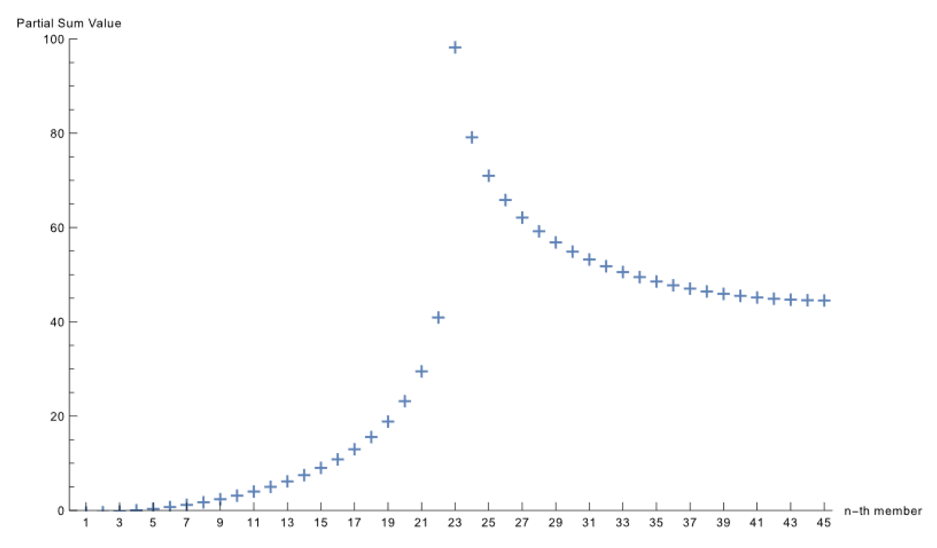
It is a somewhat surprising result considering that the only rational addend is tan 45° while the other addends are irrational. Furthermore, the fact that the number 45 as the sum of tangent values is an integer is not due to any elimination during the addition, as can be observed from both a sequence graph, see Figure 1 and partial sums, see Figure 2. The occurrence of the integer 45 at the very end may be seen as a miracle by the students.

Hence, it is worth examining this phenomenon more closely by means of high school mathematics; mathematical software helps to motivate high school students to delve deep into mathematics here [7].

3. Mathematical Background

Prove that ${\sum }_{n=0}^{44}{\tan (1+4n)}^{°}=\tan 1^{°}+\tan 5^{°}+\tan 9^{°}+\cdots +\tan {177}^{°}=45.$

Proof. 

For $x\in \left\{1, 5, 9 ,\dots ,177\right\}$ holds

$45x\equiv 45\left(mod180\right)$.

Because the tangent function is a periodical function with a period of 180°, the following applies [8]:

If $x\in \left\{1^{°},5^{°},9^{°},\dots ,{177}^{°}\right\}$, then $\tan 45x=\tan {45}^{°}=1$. By breaking down individual parts:

$\tan 45(1°)=\tan 45°, \tan 45(5°)=\tan 225°=\tan 45°, \tan 45\left(9°\right)=\tan 405°=\tan 45°,\dots ,\tan 45(177°)=\tan 7965°=\tan 45°$.

Let us think further in this manner.

Similar to the well-known double-angle formula $\tan 2x=\frac{2\tan x}{(1-{\tan }^{2}x)}$, there is an n-multiple-angle formula, [9,10]. For n = 45, the formula is

$$\tan 45x=\frac{\left(\genfrac{}{}{0pt}{}{45}{1}\right){\tan }^{1}x-\left(\genfrac{}{}{0pt}{}{45}{3}\right){\tan }^{3}x+\cdots -\left(\genfrac{}{}{0pt}{}{45}{43}\right){\tan }^{43}x+\left(\genfrac{}{}{0pt}{}{45}{45}\right){\tan }^{45}x}{\left(\genfrac{}{}{0pt}{}{45}{0}\right)1-\left(\genfrac{}{}{0pt}{}{45}{2}\right){\tan }^{2}x+\cdots -\left(\genfrac{}{}{0pt}{}{45}{42}\right){\tan }^{42}x+\left(\genfrac{}{}{0pt}{}{45}{44}\right){\tan }^{44}x},$$

and the general multiple-angle formula is as follows:

$$\tan \mathrm{n}x=\frac{{\sum }_{\mathrm{k} \mathrm{odd}}^{\mathrm{n}}(-1{)}^{\frac{\mathrm{k}-1}{2}}\left(\begin{array}{c}\mathrm{n}\\ \mathrm{k}\end{array}\right){\tan }^{\mathrm{k}}x}{{\sum }_{\mathrm{k} \mathrm{even}}^{\mathrm{n}}(-1{)}^{\frac{\mathrm{k}}{2}}\left(\begin{array}{c}\mathrm{n}\\ \mathrm{k}\end{array}\right){\tan }^{\mathrm{k}}x}.$$

There is a similar formula for the cosine function. We will use the following:

$$\cos \mathrm{n}x=\sum _{\mathrm{k}=1}^{⌊\frac{\mathrm{n}}{2}⌋+1}\frac{(-1{)}^{\mathrm{k}-1}{2}^{\mathrm{n}+1-2\mathrm{k}}·\mathrm{n}(\mathrm{n}-\mathrm{k})!}{\left(\mathrm{k}-1\right)!\left(\mathrm{n}+2-2\mathrm{k}\right)!}(\cos x{)}^{\mathrm{n}+2-2\mathrm{k}}.$$

We have shown that for $x\in \left\{1^{°},5^{°},9^{°},\dots ,{177}^{°}\right\}$, $\tan 45x=\tan {45}^{°}=1$, so we obtain the following:

$$\frac{\left(\genfrac{}{}{0pt}{}{45}{1}\right){\tan }^{1}x-\left(\genfrac{}{}{0pt}{}{45}{3}\right){\tan }^{3}x+\cdots -\left(\genfrac{}{}{0pt}{}{45}{43}\right){\tan }^{43}x+\left(\genfrac{}{}{0pt}{}{45}{45}\right){\tan }^{45}x}{\left(\genfrac{}{}{0pt}{}{45}{0}\right)1-\left(\genfrac{}{}{0pt}{}{45}{2}\right){\tan }^{2}x+\cdots -\left(\genfrac{}{}{0pt}{}{45}{42}\right){\tan }^{42}x+\left(\genfrac{}{}{0pt}{}{45}{44}\right){\tan }^{44}x}=1, \mathrm{that} \mathrm{is}$$

$\left(\begin{array}{c}45\\ 1\end{array}\right){\tan }^{1}x-\left(\begin{array}{c}45\\ 3\end{array}\right){\tan }^{3}x+\cdots -\left(\begin{array}{c}45\\ 43\end{array}\right){\tan }^{43}x+\left(\begin{array}{c}45\\ 45\end{array}\right){\tan }^{45}x=\left(\begin{array}{c}45\\ 0\end{array}\right)1-\left(\begin{array}{c}45\\ 2\end{array}\right){\tan }^{2}x+\cdots -\left(\begin{array}{c}45\\ 42\end{array}\right){\tan }^{42}x+\left(\begin{array}{c}45\\ 44\end{array}\right){\tan }^{44}x$.

Thus, ${\tan }^{45}x-45{\tan }^{44}x+\cdots +45\tan x-1=0$ for $x\in \left\{1^{°},5^{°},9^{°},\dots ,{177}^{°}\right\}.$

Using the substitution $y=\tan x$, we can say that the left-hand side of this equation is the normed polynomial function of degree 45:

$$y^{45}-45y^{44}+\cdots +45y-1,$$

and its 45 roots (see the Fundamental Theorem of Algebra) are $\tan 1^{°}, \tan 5^{°}, \tan 9^{°},\dots ,\tan {177}^{°}$, as we have explained above.

Finally, the first equality of Vieta’s formula for polynomial $y^n+a_1{y}^{n-1}+\cdots +a_{n-1}y+a_n$ (over the field of complex numbers) states that if $y_1,y_2,y_3\dots , y_n$ are its roots, then

$$y_1+y_2+y_3\dots +y_n=-a_1.$$

Therefore, we obtain

$$\tan 1^{°}+\tan 5^{°}+\tan 9^{°}+\cdots +\tan {177}^{°}=\sum _{n=0}^{44}{\tan \left(1+4n\right)}^{°}=45,$$

(1)

quod erat demonstrandum. □

If we use the last equality of Vieta’s formula, namely

$$y_1{y}_2{y}_3\dots y_n={\left(-1\right)}^n{a}_n,$$

we obtain the product of the following tangent values:

$$\tan 1^{°}\tan 5^{°}\tan 9^{°}\dots \tan {177}^{°}={\left(-1\right)}^{45}\left(-1\right)=1.$$

(2)

In the next section, we return to Wolfram Mathematica.

4. Follow-Up Problems

What is the value of the product

$${\prod }_{n=0}^{44}{\tan \left(1+4n\right)}^{°}=\tan 1^{°}\tan 5^{°}\tan 9^{°}\dots \tan {177}^{°}?$$

Explanation	e.g.,
# of the factor	3
Angle value	9°
tan (angle)°	0.15838
Partial Product of angle degrees	0.00024187

$\#: 1 \mathrm{Angle}: 1^{\circ }\mathrm{Tan}[ 1^{\circ } ]: 0.017455 \mathrm{PartProduct} \mathrm{of} 1 \mathrm{degrees}: 0.0174555$

$\#: 2 \mathrm{Angle}: 5^{\circ }\mathrm{Tan}[ 5^{\circ } ]: 0.087489 \mathrm{PartProduct} \mathrm{of} 5 \mathrm{degrees}: 0.0015271$

$\#: 3 \mathrm{Angle}: 9^{\circ }\mathrm{Tan}[ 9^{\circ } ]: 0.15838 \mathrm{PartProduct} \mathrm{of} 9 \mathrm{degrees}: 0.00024187$

$\#: 4 \mathrm{Angle}: {13}^{\circ }\mathrm{Tan}[ {13}^{\circ } ]: 0.23087 \mathrm{PartProduct} \mathrm{of} 13 \mathrm{degrees}: 0.000055841$

$\#: 5 \mathrm{Angle}: {17}^{\circ }\mathrm{Tan}[ {17}^{\circ } ]: 0.30573 \mathrm{PartProduct} \mathrm{of} 17 \mathrm{degrees}: 0.000017072$

$\#: 6 \mathrm{Angle}: {21}^{\circ }\mathrm{Tan}[ {21}^{\circ } ]: 0.38386 \mathrm{PartProduct} \mathrm{of} 21 \mathrm{degrees}: 6.55339\times {10}^{-6}$

$\#: 7 \mathrm{Angle}: {25}^{\circ }\mathrm{Tan}[ {25}^{\circ } ]: 0.46631 \mathrm{PartProduct} \mathrm{of} 25 \mathrm{degrees}: 3.05589\times {10}^{-6}$

$\#: 8 \mathrm{Angle}: {29}^{\circ }\mathrm{Tan}[ {29}^{\circ } ]: 0.55431 \mathrm{PartProduct} \mathrm{of} 29 \mathrm{degrees}: 1.693911\times {10}^{-6}$

$\#: 9 \mathrm{Angle}: {33}^{\circ }\mathrm{Tan}[ {33}^{\circ } ]: 0.64941 \mathrm{PartProduct} \mathrm{of} 33 \mathrm{degrees}: 1.100039\times {10}^{-6}$

$\#: 10 \mathrm{Angle}: {37}^{\circ }\mathrm{Tan}[ {37}^{\circ } ]: 0.75355 \mathrm{PartProduct} \mathrm{of} 37 \mathrm{degrees}: 8.289391\times {10}^{-7}$

$\#: 11 \mathrm{Angle}: {41}^{\circ }\mathrm{Tan}[ {41}^{\circ } ]: 0.86929 \mathrm{PartProduct} \mathrm{of} 41 \mathrm{degrees}: 7.205857 \times {10}^{-7}$

$\#: 12 \mathrm{Angle}: {45}^{\circ }\mathrm{Tan}[ {45}^{\circ } ]: 1.0000 \mathrm{PartProduct} \mathrm{of} 45 \mathrm{degrees}: 7.205857\times {10}^{-7}$

$\#: 13 \mathrm{Angle}: {49}^{\circ }\mathrm{Tan}[ {49}^{\circ } ]: 1.1504 \mathrm{PartProduct} \mathrm{of} 49 \mathrm{degrees}: 8.289391\times {10}^{-7}$

$\#: 14 \mathrm{Angle}: {53}^{\circ }\mathrm{Tan}[ {53}^{\circ } ]: 1.3270 \mathrm{PartProduct} \mathrm{of} 53 \mathrm{degrees}: 1.100039\times {10}^{-6}$

$\#: 15 \mathrm{Angle}: {57}^{\circ }\mathrm{Tan}[ {57}^{\circ } ]: 1.5399 \mathrm{PartProduct} \mathrm{of} 57 \mathrm{degrees}: 1.693911\times {10}^{-6}$

$\#: 16 \mathrm{Angle}: {61}^{\circ }\mathrm{Tan}[ {61}^{\circ } ]: 1.8040 \mathrm{PartProduct} \mathrm{of} 61 \mathrm{degrees}: 3.055898\times {10}^{-6}$

$\#: 17 \mathrm{Angle}: {65}^{\circ }\mathrm{Tan}[ {65}^{\circ } ]: 2.1445 \mathrm{PartProduct} \mathrm{of} 65 \mathrm{degrees}: 6.553394\times {10}^{-6}$

$\#: 18 \mathrm{Angle}: {69}^{\circ }\mathrm{Tan}[ {69}^{\circ } ]: 2.6051 \mathrm{PartProduct} \mathrm{of} 69 \mathrm{degrees}: 0.000017072$

$\#: 19 \mathrm{Angle}: {73}^{\circ }\mathrm{Tan}[ {73}^{\circ } ]: 3.2709 \mathrm{PartProduct} \mathrm{of} 73 \mathrm{degrees}: 0.000055841$

$\#: 20 \mathrm{Angle}: {77}^{\circ }\mathrm{Tan}[ {77}^{\circ } ]: 4.3315 \mathrm{PartProduct} \mathrm{of} 77 \mathrm{degrees}: 0.00024187$

$\#: 21 \mathrm{Angle}: {81}^{\circ }\mathrm{Tan}[ {81}^{\circ } ]: 6.3138 \mathrm{PartProduct} \mathrm{of} 81 \mathrm{degrees}: 0.0015271$

$\#: 22 \mathrm{Angle}: {85}^{\circ }\mathrm{Tan}[ {85}^{\circ } ]: 11.430 \mathrm{PartProduct} \mathrm{of} 85 \mathrm{degrees}: 0.017455$

$\#: 23 \mathrm{Angle}: {89}^{\circ }\mathrm{Tan}[ {89}^{\circ } ]: 57.290 \mathrm{PartProduct} \mathrm{of} 89 \mathrm{degrees}: 1.000$

$\#: 24 \mathrm{Angle}: {93}^{\circ }\mathrm{Tan}[ {93}^{\circ } ]: -19.081 \mathrm{PartProduct} \mathrm{of} 93 \mathrm{degrees}: -19.081$

$\#: 25 \mathrm{Angle}: {97}^{\circ }\mathrm{Tan}[ {97}^{\circ } ]: -8.1443 \mathrm{PartProduct} \mathrm{of} 97 \mathrm{degrees}: 155.40$

$\#: 26 \mathrm{Angle}: {101}^{\circ }\mathrm{Tan}[ {101}^{\circ } ]: -5.1446 \mathrm{PartProduct} \mathrm{of} 101 \mathrm{degrees}: -799.48$

$\#: 27 \mathrm{Angle}: {105}^{\circ }\mathrm{Tan}[ {105}^{\circ } ]: -3.7321 \mathrm{PartProduct} \mathrm{of} 105 \mathrm{degrees}: 2983.7$

$\#: 28 \mathrm{Angle}: {109}^{\circ }\mathrm{Tan}[ {109}^{\circ } ]: -2.9042 \mathrm{PartProduct} \mathrm{of} 109 \mathrm{degrees}: -8665.3$

$\#: 29 \mathrm{Angle}: {113}^{\circ }\mathrm{Tan}[ {113}^{\circ } ]: -2.3559 \mathrm{PartProduct} \mathrm{of} 113 \mathrm{degrees}: \mathrm{20,414}.$

$\#: 30 \mathrm{Angle}: {117}^{\circ }\mathrm{Tan}[ {117}^{\circ } ]: -1.9626 \mathrm{PartProduct} \mathrm{of} 117 \mathrm{degrees}: -\mathrm{40,065}.$

$\#: 31 \mathrm{Angle}: {121}^{\circ }\mathrm{Tan}[ {121}^{\circ } ]: -1.6643 \mathrm{PartProduct} \mathrm{of} 121 \mathrm{degrees}: \mathrm{66,680}.$

$\#: 32 \mathrm{Angle}: {125}^{\circ }\mathrm{Tan}[ {125}^{\circ } ]: -1.4281 \mathrm{PartProduct} \mathrm{of} 125 \mathrm{degrees}: -\mathrm{95,228}.$

$\#: 33 \mathrm{Angle}: {129}^{\circ }\mathrm{Tan}[ {129}^{\circ } ]: -1.2349 \mathrm{PartProduct} \mathrm{of} 129 \mathrm{degrees}: \mathrm{117,600}.$

$\#: 34 \mathrm{Angle}: {133}^{\circ }\mathrm{Tan}[ {133}^{\circ } ]: -1.0724 \mathrm{PartProduct} \mathrm{of} 133 \mathrm{degrees}: -\mathrm{126,110}.$

$\#: 35 \mathrm{Angle}: {137}^{\circ }\mathrm{Tan}[ {137}^{\circ } ]: -0.93252 \mathrm{PartProduct} \mathrm{of} 137 \mathrm{degrees}: \mathrm{117,600}.$

$\#: 36 \mathrm{Angle}: {141}^{\circ }\mathrm{Tan}[ {141}^{\circ } ]: -0.80978 \mathrm{PartProduct} \mathrm{of} 141 \mathrm{degrees}: -\mathrm{95,228}.$

$\#: 37 \mathrm{Angle}: {145}^{\circ }\mathrm{Tan}[ {145}^{\circ } ]: -0.70021 \mathrm{PartProduct} \mathrm{of} 145 \mathrm{degrees}: \mathrm{66,680}.$

$\#: 38 \mathrm{Angle}: {149}^{\circ }\mathrm{Tan}[ {149}^{\circ } ]: -0.60086 \mathrm{PartProduct} \mathrm{of} 149 \mathrm{degrees}: -\mathrm{40,065}.$

$\#: 39 \mathrm{Angle}: {153}^{\circ }\mathrm{Tan}[ {153}^{\circ } ]: -0.50953 \mathrm{PartProduct} \mathrm{of} 153 \mathrm{degrees}: \mathrm{20,414}.$

$\#: 40 \mathrm{Angle}: {157}^{\circ }\mathrm{Tan}[ {157}^{\circ } ]: -0.42447 \mathrm{PartProduct} \mathrm{of} 157 \mathrm{degrees}: -8665.3$

$\#: 41 \mathrm{Angle}: {161}^{\circ }\mathrm{Tan}[ {161}^{\circ } ]: -0.34433 \mathrm{PartProduct} \mathrm{of} 161 \mathrm{degrees}: 2983.7$

$\#: 42 \mathrm{Angle}: {165}^{\circ }\mathrm{Tan}[ {165}^{\circ } ]: -0.26795 \mathrm{PartProduct} \mathrm{of} 165 \mathrm{degrees}: -799.48$

$\#: 43 \mathrm{Angle}: {169}^{\circ }\mathrm{Tan}[ {169}^{\circ } ]: -0.19438 \mathrm{PartProduct} \mathrm{of} 169 \mathrm{degrees}: 155.40$

$\#: 44 \mathrm{Angle}: {173}^{\circ }\mathrm{Tan}[ {173}^{\circ } ]: -0.12278 \mathrm{PartProduct} \mathrm{of} 173 \mathrm{degrees}: -19.081$

$\#: 45 \mathrm{Angle}: {177}^{\circ }\mathrm{Tan}[ {177}^{\circ } ]: -0.052408 \mathrm{PartProduct} \mathrm{of} 177 \mathrm{degrees}: 1.0000$

The product of the sequence is

1.000000000000000000000000000000000000000000000000000000000000000000000000000000000000000000000000000000000000000000000000000000000000000000000000000000000000000000000000000000000000000000000000000000000000000000000000000000000000000000000000000000000000000000000000000000000000000000000000000000000000.

The mathematical software, therefore, shows us that the product could have a value of 1. That is the correct result, as we have already shown in the Mathematics environment—see the last equality of Vieta’s formula $y_1{y}_2{y}_3\dots y_n={(-1)}^n{a}_n$.

Let us now look at the case of tan 2x. From now on, we will use Wolfram Mathematica notation since the syntax from this notebook is perfectly readable, and there are no ambiguities.

tangentMultipleAngle[n_, x_] :=

Module[{oddSum, evenSum},

oddSum = Sum[(−1)^((k − 1)/2) Binomial[n, k] Tan[x]^k, {k, 1, n, 2}];

evenSum = Sum[(−1)^(k/2) Binomial[n, k] Tan[x]^k, {k, 0, n, 2}];

oddSum/evenSum]

result = tangentMultipleAngle[2, x]

$\frac{2\mathrm{T}\mathrm{a}\mathrm{n}\left[x\right]}{1-{\mathrm{T}\mathrm{a}\mathrm{n}\left[x\right]}^2}$

This code defines a function called tangentMultipleAngle, which takes two arguments, n and x. Inside the function, there are two local variables defined: oddSum and evenSum. The oddSum variable is assigned the value of the sum of a series of terms.

The series is calculated using the Sum function, which takes three arguments: the expression to sum, the index variable, and the range of values for the index variable. In this case, the expression that is being summed is (−1)^((k − 1)/2)$·$Binomial[n, k]$·$Tan[x]^k, the index variable is k, and the range of values for k is from 1 to n with a step size of 2. The evenSum variable is assigned the value of another sum of terms calculated in a similar way as the oddSum variable but with a different expression being summed: (−1)^(k/2)$·$Binomial[n, k]$·$Tan[x]^k. The range of values for k in the case of evenSum is from 0 to n with a step size of 2.

Finally, the function returns the value of oddSum divided by evenSum.

The code also includes a usage example where the variables n and x are cleared, and the function tangentMultipleAngle is called with the arguments 2 and x. The result of the function call is assigned to the result variable [11].

eq = Tan[2 x] == $\frac{2\mathrm{T}\mathrm{a}\mathrm{n}\left[x\right]}{1-{\mathrm{T}\mathrm{a}\mathrm{n}\left[x\right]}^2}$; (*Verification of the multiple angel formula*)

Simplify[eq]

True

The code starts by defining an equation eq using the $==$ operator, which checks if the left-hand side is equal to the right-hand side. In this case, the equation is Tan [2x] $==$ (2 Tan[x])/(1 − Tan[x]^2).

The equation represents the verification of the multiple-angle formula for the tangent function. The multiple-angle formula states that Tan [2x] can be expressed in terms of Tan[x] using the equation (2 Tan[x])/(1 − Tan[x]^2).

The Simplify function is then used to simplify the equation eq. The Simplify function is a built-in function in Mathematica that attempts to simplify mathematical expressions. In this case, it simplifies the equation by applying various algebraic simplifications and trigonometric identities.

The result of the code is a simplified equation, which is the same as the original equation eq. This indicates that the multiple-angle formula for the tangent function is verified.

For x∈{1 Degree, 91 Degrees} holds that 2x ≡ 2(mod 180)

Tan[2x] = $\frac{2\mathrm{T}\mathrm{a}\mathrm{n}\left[x\right]}{1-{\mathrm{T}\mathrm{a}\mathrm{n}\left[x\right]}^2}$, Tan[2×1 Degree] = $\frac{2\mathrm{T}\mathrm{a}\mathrm{n}\left[1\mathrm{D}\mathrm{e}\mathrm{g}\mathrm{r}\mathrm{e}\mathrm{e}\right]}{1-{\mathrm{T}\mathrm{a}\mathrm{n}\left[1\mathrm{D}\mathrm{e}\mathrm{g}\mathrm{r}\mathrm{e}\mathrm{e}\right]}^2}$ and

Tan[2×91 Degree] = Tan[2 Degree] = $\frac{2\mathrm{T}\mathrm{a}\mathrm{n}\left[91\mathrm{D}\mathrm{e}\mathrm{g}\mathrm{r}\mathrm{e}\mathrm{e}\right]}{1-{\mathrm{T}\mathrm{a}\mathrm{n}\left[91\mathrm{D}\mathrm{e}\mathrm{g}\mathrm{r}\mathrm{e}\mathrm{e}\right]}^2}$

Substitution y1 := Tan[1 Degree], then Tan[2 Degree](1 − y12) = 2y1, i.e. −y12 − (2/Tan[2 Degree])y1 + 1 = 0.

Similarly, substitution y2 := Tan[91 Degree], then Tan[2 Degree](1 − y22) = 2y2,i.e. −y22 − (2/Tan[2 Degree])y2 + 1 = 0. Thus both y1 and y2 are roots of the equationy2 +(2/Tan[2 Degree])y − 1 = 0. According to the Vieta’s formula the following identities should be valid: the sum y1 + y2 = −2/Tan[2 Degree]

(= −57.27250656583120710151301864189285015590342064630405120) and the product y1y2 = −1.

N[−2/Tan[2 Degree], 55]

−57.27250656583120710151301864189285015590342064630405120

N[Tan[1 Degree] + Tan[91 Degree], 55]

−57.27250656583120710151301864189285015590342064630405120

N[Tan[1 Degree]*Tan[91 Degree], 55]

−1.000000000000000000000000000000000000000000000000000000

Then, the sum and the product look OK.

Why OK? It corresponds to the Vieta’s equalities; the equation appears as follows:

$$y^2+\frac{2}{\tan 2°}y-1=0$$

$y_1+y_2=-\frac{2}{\tan 2°}$ and $y_1{y}_2=-1$

Tan[1 Degree] + Tan[91 Degree] + 2/Tan[2 Degree] // N

$-3.434752482434078\times {10}^{-15}$

We must always be careful because even though the values $-\frac{2}{\tan 2°}$ and $(\tan 1°+\tan 91°)$ look equal (always having the value $-$57.272506565831207 10151301864189285015590342064630405119), their difference is not exactly zero:

Tan[1 Degree] + Tan[91 Degree] - (-2/Tan[2 Degree]) // N

$-3.434752482434078\times {10}^{-15}$

We will now focus on cases where the sum of the sequence of tangent values is rational (even an integer).

From the general tangent multiple-angle formula $\tan \mathrm{n}x=\frac{{\sum }_{\mathrm{k} \mathrm{odd}}^{\mathrm{n}}(-1{)}^{\frac{\mathrm{k}-1}{2}}\left(\begin{array}{c}\mathrm{n}\\ \mathrm{k}\end{array}\right){\tan }^{\mathrm{k}}x}{{\sum }_{\mathrm{k} \mathrm{even}}^{\mathrm{n}}(-1{)}^{\frac{\mathrm{k}}{2}}\left(\begin{array}{c}\mathrm{n}\\ \mathrm{k}\end{array}\right){\tan }^{\mathrm{k}}x}$, it follows that for the sum to be a rational number, nx must be congruent to $45 \left(mod 180\right), \mathrm{i}.\mathrm{e}.,$ $\mathrm{n}x\equiv 45(mod 180)$. Using this assumption with the following computer yields

number = 45;

For[divisor = 1, divisor ≤ number, divisor++,

If[Mod[number, divisor] == 0, quotient = number/divisor;

quotient180 = 180/divisor;

sum = 0;

degreeStep = quotient180; (*Angle increment between consecutive terms*)

startDegree = quotient; (*Starting angle in degrees*)

endDegree = 180 − degreeStep + startDegree; (*Ending angle in degrees*)

Do[angle = degree*Degree;

(*Convert the angle to radians*) term = Tan[angle];

sum += term;

{degree, startDegree, endDegree, degreeStep},

{degree, startDegree, endDegree, degreeStep}];

Print[“number of addends:”, 1 + (endDegree − startDegree)/degreeStep,

“ startDegree: ”, startDegree, “ degreeStep: ”, degreeStep,

“ endDegree: ”, endDegree, “ The sum of the sequence is: ”, N[sum]]]]

We obtain

number of addends:1 startDegree: 45 degreeStep: 180 endDegree: 45

The sum of the sequence is 1.

number of addends:3 startDegree: 15 degreeStep: 60 endDegree: 135

The sum of the sequence is 3.

number of addends:5 startDegree: 9 degreeStep: 36 endDegree: 153

The sum of the sequence is 5.

number of addends:9 startDegree: 5 degreeStep: 20 endDegree: 165

The sum of the sequence is 9.

number of addends:15 startDegree: 3 degreeStep: 12 endDegree: 171

The sum of the sequence is 15.

number of addends:45 startDegree: 1 degreeStep: 4 endDegree: 177

The sum of the sequence is 45.

In other words, Wolfram Mathematica suggested the following might be true:

• ${\sum }_{n=0}^0{\tan \left(45+180n\right)}^{°}=1,$
• ${\sum }_{n=0}^2{\tan \left(15+60n\right)}^{°}=3,$
• ${\sum }_{n=0}^4{\tan \left(9+36n\right)}^{°}=5,$
• ${\sum }_{n=0}^8{\tan \left(5+20n\right)}^{°}=9,$
• ${\sum }_{n=0}^{14}{\tan \left(3+12n\right)}^{°}=15,$
• ${\sum }_{n=0}^{44}{\tan \left(1+4n\right)}^{°}=45.$

We have already shown that equality 6 holds in Wolfram Mathematica and proved it mathematically. The equalities 1 to 5 can be shown within Mathematica and proved mathematically in the same way.

Let us conduct this for equality 2. (Equality 1 is trivial: ${\sum }_{n=0}^0{\tan \left(45+180 n\right)}^{°}=\tan 45°=1.$)

Thus, we calculate in Mathematica ${\sum }_{n=0}^2{\tan \left(15+60 n\right)}^{°}$:

N[Tan[15 Degree] + Tan[75 Degree] + Tan[135 Degree], 50]

3.0000000000000000000000000000000000000000000000000

Now, we proved the result mathematically. (Again, we will use Wolfram Mathematica notation.)

Tan[3x] − for the sum’ s value 3

For x∈{15 Degrees, 75 Degrees, 135 Degrees} holds that 3x ≡ 45(mod 180)

Tan[3x] = $\frac{\left(\begin{array}{c}3\\ 1\end{array}\right)\mathrm{T}\mathrm{a}\mathrm{n}[x]-\left(\begin{array}{c}3\\ 3\end{array}\right){\mathrm{T}\mathrm{a}\mathrm{n}\left[x\right]}^3}{\left(\begin{array}{c}3\\ 0\end{array}\right)-\left(\begin{array}{c}3\\ 2\end{array}\right){\mathrm{T}\mathrm{a}\mathrm{n}\left[x\right]}^2}$, thus

Tan[3×15 Degree] = $\frac{\left(\begin{array}{c}3\\ 1\end{array}\right)\mathrm{T}\mathrm{a}\mathrm{n}[15\mathrm{D}\mathrm{e}\mathrm{g}\mathrm{r}\mathrm{e}\mathrm{e}]-\left(\begin{array}{c}3\\ 3\end{array}\right){\mathrm{T}\mathrm{a}\mathrm{n}\left[15\mathrm{D}\mathrm{e}\mathrm{g}\mathrm{r}\mathrm{e}\mathrm{e}\right]}^3}{\left(\begin{array}{c}3\\ 0\end{array}\right)-\left(\begin{array}{c}3\\ 2\end{array}\right){\mathrm{T}\mathrm{a}\mathrm{n}\left[15\mathrm{D}\mathrm{e}\mathrm{g}\mathrm{r}\mathrm{e}\mathrm{e}\right]}^2}$.

Tan[3×75 Degree] = $\frac{\left(\begin{array}{c}3\\ 1\end{array}\right)\mathrm{T}\mathrm{a}\mathrm{n}[75\mathrm{D}\mathrm{e}\mathrm{g}\mathrm{r}\mathrm{e}\mathrm{e}]-\left(\begin{array}{c}3\\ 3\end{array}\right){\mathrm{T}\mathrm{a}\mathrm{n}\left[75\mathrm{D}\mathrm{e}\mathrm{g}\mathrm{r}\mathrm{e}\mathrm{e}\right]}^3}{\left(\begin{array}{c}3\\ 0\end{array}\right)-\left(\begin{array}{c}3\\ 2\end{array}\right){\mathrm{T}\mathrm{a}\mathrm{n}\left[75\mathrm{D}\mathrm{e}\mathrm{g}\mathrm{r}\mathrm{e}\mathrm{e}\right]}^2}$ and

Tan[3×135 Degree] = $\frac{\left(\begin{array}{c}3\\ 1\end{array}\right)\mathrm{T}\mathrm{a}\mathrm{n}[135\mathrm{D}\mathrm{e}\mathrm{g}\mathrm{r}\mathrm{e}\mathrm{e}]-\left(\begin{array}{c}3\\ 3\end{array}\right){\mathrm{T}\mathrm{a}\mathrm{n}\left[135\mathrm{D}\mathrm{e}\mathrm{g}\mathrm{r}\mathrm{e}\mathrm{e}\right]}^3}{\left(\begin{array}{c}3\\ 0\end{array}\right)-\left(\begin{array}{c}3\\ 2\end{array}\right){\mathrm{T}\mathrm{a}\mathrm{n}\left[135\mathrm{D}\mathrm{e}\mathrm{g}\mathrm{r}\mathrm{e}\mathrm{e}\right]}^2}$

Apparently, Tan[3×15 Degree] = Tan[3×75 Degree] = Tan[3×135 Degree] = Tan[45 Degree] = 1.

Substitution y1 := Tan[15 Degree], then $\left(\begin{array}{c}3\\ 3\end{array}\right)$y13 − $\left(\begin{array}{c}3\\ 2\end{array}\right)$Tan[3×15 Degree]y12) − $\left(\begin{array}{c}3\\ 1\end{array}\right)$y1 + $\left(\begin{array}{c}3\\ 0\end{array}\right)$Tan[3×15 Degree] = 0, i.e. y13 − 3y12 − 3y1 + 1 = 0.

Similarly, the substitution y2 := Tan[75 Degree] leads to the cubic equation y23 − 3y22 − 3y2 + 1 = 0, and finally, the substitution y3 := Tan[135 Degree] leads to the cubic equation y33 − 3y32 − 3y3 + 1 = 0.

Thus y1, y2 and y3 are roots of the equation y3 − 3y2 − 3y + 1 = 0. According to the Vieta’s formula the following identities should be valid: the sum y1 + y2 + y3 = 3 and the product y1y2y3 = −1.

Since we also included the product here, let us calculate it in Mathematica as well.

N[Tan[15 Degree] * Tan[75 Degree] * Tan[135 Degree], 50]

−1.0000000000000000000000000000000000000000000000000

Note here that the irrational values tan 15° and tan 75° can be easily expressed in Mathematica as follows, but we could also find the roots of the equation

$$y^3-3y^2-3y+1=0:$$

Solve[y^3 − 3y^2 − 3y + 1 == 0, y]

$\left\{\right\{y\to -1\},\{y\to 2-\sqrt{3}\},\{y\to 2+\sqrt{3}\left\}\right\}$

{Tan[15 Degree], Tan[75 Degree], Tan[135 Degree]}

{$2-\sqrt{3}$, $2+\sqrt{3}$, $-1$}

$\left\{\right\{y\to -1\},\{y\to 2-\sqrt{3}\},\{y\to 2+\sqrt{3}\left\}\right\}$

5. Discussion

The following reflection can initiate a discussion about the results obtained via mathematical software. More intriguing explorations can follow.

Let us show in connection with the sum of tangent values that the results obtained with the help of mathematical software really motivate us to mathematically explain some “regularities” and delve deeper into mathematics. For example, we may want to find out for which positive integers p the following is true:

$$\sum _{n=0}^{44}{\tan \left(1+4pn\right)}^{°}=45.$$

Wolfram Mathematica shows

sum45ValuesOfP = { };

Do[sum = N[Sum[Tan[(π/180) (1 + p*4 i)], {i, 0, 44}]];

If[sum == 45, Print[“Sum = 45 for 4*p, where p =”, p];

AppendTo[sum45ValuesOfP, p];,

Print[“Sum =”, sum, “for 4*p, where p =”, p];], {p, 1, 100}]

Print[“Values of p for which the sum is 45:”, sum45ValuesOfP];

Sum = 45 for 4*p, where p = 1

Sum = 45 for 4*p, where p = 2

Sum = 12.0577 for 4*p, where p = 3

Sum = 45 for 4*p, where p = 4

Sum = 7.1273 for 4*p, where p = 5

Sum = 12.0577 for 4*p, where p = 6

Sum = 45 for 4*p, where p = 7

Sum = 45 for 4*p, where p = 8

Sum = 3.93699 for 4*p, where p = 9

Sum = 7.1273 for 4*p, where p = 10

Sum = 45 for 4*p, where p = 11

Sum = 12.0577 for 4*p, where p = 12

Sum = 45 for 4*p, where p = 13

Sum = 45 for 4*p, where p = 14

Sum = 2.35835 for 4*p, where p = 15

Sum = 45 for 4*p, where p = 16

Sum = 45 for 4*p, where p = 17

Sum = 3.93699 for 4*p, where p = 18

Sum = 45 for 4*p, where p = 19

Sum = 7.1273 for 4*p, where p = 20

Sum = 12.0577 for 4*p, where p = 21

Sum = 45 for 4*p, where p = 22

Sum = 45 for 4*p, where p = 23

Sum = 12.0577 for 4*p, where p = 24

Sum = 7.1273 for 4*p, where p = 25

Sum = 45 for 4*p, where p = 26

Sum = 3.93699 for 4*p, where p = 27

Sum = 45 for 4*p, where p = 28

Sum = 45 for 4*p, where p = 29

Sum = 2.35835 for 4*p, where p = 30

Sum = 45 for 4*p, where p = 31

Sum = 45 for 4*p, where p = 32

Sum = 12.0577 for 4*p, where p = 33

Sum = 45 for 4*p, where p = 34

Sum = 7.1273 for 4*p, where p = 35

Sum = 3.93699 for 4*p, where p = 36

Sum = 45 for 4*p, where p = 37

Sum = 45 for 4*p, where p = 38

Sum = 12.0577 for 4*p, where p = 39

Sum = 7.1273 for 4*p, where p = 40

Sum = 45 for 4*p, where p = 41

Sum = 12.0577 for 4*p, where p = 42

Sum = 45 for 4*p, where p = 43

Sum = 45 for 4*p, where p = 44

Sum = 0.785478 for 4*p, where p = 45

Sum = 45 for 4*p, where p = 46

Sum = 45 for 4*p, where p = 47

Sum = 12.0577 for 4*p, where p = 48

Sum = 45 for 4*p, where p = 49

Sum = 7.1273 for 4*p, where p = 50

Sum = 12.0577 for 4*p, where p = 51

Sum = 45 for 4*p, where p = 52

Sum = 45 for 4*p, where p = 53

Sum = 3.93699 for 4*p, where p = 54

Sum = 7.1273 for 4*p, where p = 55

Sum = 45 for 4*p, where p = 56

Sum = 12.0577 for 4*p, where p = 57

Sum = 45 for 4*p, where p = 58

Sum = 45 for 4*p, where p = 59

Sum = 2.35835 for 4*p, where p = 60

Sum = 45 for 4*p, where p = 61

Sum = 45 for 4*p, where p = 62

Sum = 3.93699 for 4*p, where p = 63

Sum = 45 for 4*p, where p = 64

Sum = 7.1273 for 4*p, where p = 65

Sum = 12.0577 for 4*p, where p = 66

Sum = 45 for 4*p, where p = 67

Sum = 45 for 4*p, where p = 68

Sum = 12.0577 for 4*p, where p = 69

Sum = 7.1273 for 4*p, where p = 70

Sum = 45 for 4*p, where p = 71

Sum = 3.93699 for 4*p, where p = 72

Sum = 45 for 4*p, where p = 73

Sum = 45 for 4*p, where p = 74

Sum = 2.35835 for 4*p, where p = 75

Sum = 45 for 4*p, where p = 76

Sum = 45 for 4*p, where p = 77

Sum = 12.0577 for 4*p, where p = 78

Sum = 45 for 4*p, where p = 79

Sum = 7.1273 for 4*p, where p = 80

Sum = 3.93699 for 4*p, where p = 81

Sum = 45 for 4*p, where p = 82

Sum = 45 for 4*p, where p = 83

Sum = 12.0577 for 4*p, where p = 84

Sum = 7.1273 for 4*p, where p = 85

Sum = 45 for 4*p, where p = 86

Sum = 12.0577 for 4*p, where p = 87

Sum = 45 for 4*p, where p = 88

Sum = 45 for 4*p, where p = 89

Sum = 0.785478 for 4*p, where p = 90

Sum = 45 for 4*p, where p = 91

Sum = 45 for 4*p, where p = 92

Sum = 12.0577 for 4*p, where p = 93

Sum = 45 for 4*p, where p = 94

Sum = 7.1273 for 4*p, where p = 95

Sum = 12.0577 for 4*p, where p = 96

Sum = 45 for 4*p, where p = 97

Sum = 45 for 4*p, where p = 98

Sum = 3.93699 for 4*p, where p = 99

Sum = 7.1273 for 4*p, where p = 100

Values of p for which the sum is 45:

{1,2,4,7,8,11,13,14,16,17,19,22,23,26,28,29,31,32,34,37,38,41,43,44,46,47,49,52,53,56,58,59,61,62,64,67,68,71,73,74,76,77,79,82,83,86,88,89,91,92,94,97,98}

It appears that the sequence starts with the number 1 followed by groups of eight numbers created by eight successive increments of the values 1, 2, 3, 1, 3, 2, 1, and 2. This process is repeating, i.e., the increments form a cycle $\overline{1,2,3,1,3,2,1,2}$.

1, 1 + 1 = 2, 2 + 2 = 4, 4 + 3 = 7, 7 + 1 = 8, 8 + 3 = 11, 11 + 2 = 13, 13 + 1 = 14, 14 + 2 = 16. The next group is 16 + 1 = 17, 17 + 2 = 19, 19 + 3 = 22, 22 + 1 = 23, 23 + 3 = 26, 26 + 2 = 28, 28 + 1 = 29, 29 + 2 = 31, etc.

Another topic for discussion is as follows:

Let us focus on the case where the sum of the members of a sequence is a rational number, but Wolfram Mathematica does not show the sum exactly.

However, to find such a case, we will need to look for the sum of the cosines’ values instead of the sum of tangents’ values.

We know the general cosine multiple-angle formula:

$$\cos \mathrm{n}x=\sum _{\mathrm{k}=1}^{⌊\frac{\mathrm{n}}{2}⌋+1}\frac{(-1{)}^{\mathrm{k}-1}{2}^{\mathrm{n}+1-2\mathrm{k}}·\mathrm{n}(\mathrm{n}-\mathrm{k})!}{\left(\mathrm{k}-1\right)!\left(\mathrm{n}+2-2\mathrm{k}\right)!}(\cos x{)}^{\mathrm{n}+2-2\mathrm{k}}.$$

It is easy to define a special case of this formula in Wolfram Mathematica:

cosineFormula[n_, x_] :=

Module[{result=0},

For [k = 1, k ≤ Floor[n/2] + 1, k++, result += (-1)^(k-1) * 2^(n+1-2k) * n *

Factorial[n-k]/(Factorial[k-1] * Factorial[n+2-2k]) *

(Cos[x])^(n+2-2k)];

result]

result = cosineFormula[3, x]

$-3\mathrm{C}\mathrm{o}\mathrm{s}\left[x\right]+4{\mathrm{C}\mathrm{o}\mathrm{s}\left[x\right]}^3$

This code defines a function called cosineFormula that takes two arguments: n and x. Inside the function, there is a Module that initializes a variable called result to 0.

Then, there is a For loop that iterates from k = 1 to Floor[n/2] + 1.

Inside the loop, the result variable is updated by adding a term calculated using the cosine formula.

The term is calculated as follows:

• (−1)^(k − 1) is multiplied by 2^(n + 1 − 2 k), n, and a combination of factorials.
• The combination of factorials is calculated as Factorial[n − k]/(Factorial[k − 1]*Factorial[n + 2 − 2 k]).
• Finally, the term is multiplied by (Cos[x])^(n + 2 − 2 k).

After the loop, the result variable is returned as the output of the function.

Outside the function, the cosineFormula function is called with the arguments 3 and x, and the result is assigned to the variable result [11].

For x ∈{20 Degree, 140 Degrees, 260 Degrees} holds that 3x ≡ 60(mod 360)

Cos[3x] = −3Cos[x] + 4Cos[x]3,

Cos[3×20 Degree] = Cos[60 Degree] = −3Cos[20 Degree] + 4Cos[20 Degree]3 and

Cos[3×140 Degree] = Cos[60 Degree] = −3Cos[140 Degree] + 4Cos[140Degree]3 and

Cos[3×260 Degree] = Cos[60 Degree] = -3Cos[260 Degree] + 4Cos[260Degree]3

Substitution y1 := Cos[20 Degree], then 4y13 + 0y12 − 3y1 − Cos[60 Degree] = 0, i.e. y13 + 0/4y12 − 3/4y1 − Cos[60 Degree]/4 = 0, i.e. y13 − 3/4y1 − 1/8 = 0.

Similarly, substitution y2 := Cos[140 Degree], then 4y23 + 0y22 − 3y2 − Cos[60 Degree] = 0, i.e. y23 + 0/4y22 − 3/4y2 − Cos[60 Degree]/4 = 0, i.e. y23 − 3/4y2 −1/8 = 0. And finally, substitution y3 := Cos[260 Degree], then 4y33 + 0y32 − 3y3 − Cos[60 Degree] = 0, i.e. y33 + 0/4y32 − 3/4y3 − Cos[60 Degree]/4 = 0, i.e. y33 − 3/4y3 −1/8 = 0.

Thus y1, y2 and y3 are roots of the equation y3 − 3/4y − 1/8 = 0. According to the Vieta’s formula the following identities should be valid: the sum y1 + y2 + y3 = 0 and the product y1y2y3 = 1/8.

{N[Cos[20 Degree], 50], N[Cos[140 Degree], 50], N[Cos[260 Degree], 50]}

{0.93969262078590838405410927732473146993620813426446,

−0.76604444311897803520239265055541667393583245708040,

−0.17364817766693034885171662676931479600037567718407}

Cos[20 Degree] + Cos[140 Degree] + Cos[260 Degree] // N

$8.326672684688674\times {10}^{-17}$

Cos[20 Degree] * Cos[140 Degree] * Cos[260 Degree] // N

0.125

It can be seen that the sum in Wolfram Mathematica did not come out as exactly zero. (However, the product is correct—even theoretically—and turned out to be 1/8 = 0.125.)

6. Conclusions

In this article, we have demonstrated the valuable role of symbolic computations, exemplified by the Wolfram Mathematica environment utilizing the transition from informal experimentation to formal mathematical justifications.

By providing a problem that can be easily solved using mathematical software, we have effectively induced curiosity and critical thinking in students. The result obtained from the software, although seemingly accurate, has raised doubts about its correctness due to the inherent precision limitations of numerical calculations. Therefore, the students have been motivated to seek mathematical proof to confirm the result. This encourages them to explore formal mathematics further and also to understand the principles behind the sum of irrational numbers.

The accessibility of mathematical software like Wolfram Mathematica plays a key role in encouraging students to move beyond mere computation and engage in rigorous mathematical reasoning. As educators and researchers, we advocate for the integration of such software tools into high school curricula to stimulate a passion for mathematics and nurture the mathematicians of the future.

References

- Chao, T.; Chen, J.; Star, J.R.; Dede, C. Using Digital Resources for Motivation and Engagement in Learning Mathematics: Reflections from Teachers and Students. Digit. Exp. Math. Educ. 2016, 2, 253–277. [Google Scholar] [CrossRef]
- Bailey, D.H.; Borwein, J.M.; Martin, U.; Salvy, B.; Taufer, M. Opportunities and Challenges in 21st Century Experimental Mathematical Computation: ICERM Workshop Report. 2014. Available online: https://www.davidhbailey.com/dhbpapers/ICERM-2014.pdf (accessed on 28 July 2023).
- Maron, M.J.; Ralston, P.A.; Tyler, L.D. Utilizing the symbolic capabilities of a computer algebra system. In Technology-Based Re-Engineering Engineering Education, Proceedings of Frontiers in Education FIE’96 26th Annual Conference, Salt Lake City, UT, USA, 6–9 November 1996; IEEE: New York, NY, USA, 1996; Volume 3, pp. 1089–1091. [Google Scholar] [CrossRef]
- Mourrain, B.; Prieto, H. A Framework for Symbolic and Numeric Computations; [Research Report] RR-4013; INRIA: Paris, France, 2000. [Google Scholar]
- Fischbein, E.; Jehiam, R.; Cohen, D. The concept of irrational numbers in high-school students and prospective teachers. Educ. Stud. Math. 1995, 29, 29–44. [Google Scholar] [CrossRef]
- Harrison, J. Formal Verification of Floating Point Trigonometric Functions. In Formal Methods in Computer-Aided Design. FMCAD 2000. Lecture Notes in Computer Science; Springer: Berlin/Heidelberg, Germany, 2000; Volume 1954. [Google Scholar] [CrossRef]
- Kramarenko, T.H.; Lohvynenko, Y.S. Using the Wolfram|Alpha Project to Teach Future Mathematics Teachers. CTE Workshop Proc. 2013, 1, 119–120. [Google Scholar] [CrossRef]
- Vince, J. Modular Arithmetic. In Foundation Mathematics for Computer Science; Springer: Cham, Switzerland, 2023; pp. 123–139. [Google Scholar] [CrossRef]
- Weisstein, E.W. “Multiple-Angle Formulas”. From MathWorld—A Wolfram Web Resource. Available online: https://mathworld.wolfram.com/Multiple-AngleFormulas.html (accessed on 26 July 2023).
- Weisstein, E.W. “Tangent”. From MathWorld—A Wolfram Web Resource. Available online: https://mathworld.wolfram.com/Tangent.html (accessed on 26 July 2023).
- Hastings, C.; Mischo, K.; Morrison, M. Hands-on Start to Wolfram Mathematica and Programming with the Wolfram Language, 2nd ed.; Wolfram Media: Champaign, IL, USA, 2016. [Google Scholar]
Figure 1.
Individual addends.
Figure 2.
Partial sums.
Disclaimer/Publisher’s Note: The statements, opinions and data contained in all publications are solely those of the individual author(s) and contributor(s) and not of MDPI and/or the editor(s). MDPI and/or the editor(s) disclaim responsibility for any injury to people or property resulting from any ideas, methods, instructions or products referred to in the content. |
© 2023 by the authors. Licensee MDPI, Basel, Switzerland. This article is an open access article distributed under the terms and conditions of the Creative Commons Attribution (CC BY) license (https://creativecommons.org/licenses/by/4.0/).
Share and Cite
MDPI and ACS Style
Nocar, D.; Grossman, G.; Vaško, J.; Zdráhal, T. The Accuracy of Computational Results from Wolfram Mathematica in the Context of Summation in Trigonometry. Computation 2023, 11, 222. https://doi.org/10.3390/computation11110222
AMA Style
Nocar D, Grossman G, Vaško J, Zdráhal T. The Accuracy of Computational Results from Wolfram Mathematica in the Context of Summation in Trigonometry. Computation. 2023; 11(11):222. https://doi.org/10.3390/computation11110222
Chicago/Turabian StyleNocar, David, George Grossman, Jiří Vaško, and Tomáš Zdráhal. 2023. "The Accuracy of Computational Results from Wolfram Mathematica in the Context of Summation in Trigonometry" Computation 11, no. 11: 222. https://doi.org/10.3390/computation11110222
Note that from the first issue of 2016, this journal uses article numbers instead of page numbers. See further details here.